It seems we can’t find what you’re looking for. Perhaps searching can help.
Copyright © 2025 RealBeer
It seems we can’t find what you’re looking for. Perhaps searching can help.
A Study of Fluid Flow Through A Grainbed Using a Manifold-type
Lautering System
by John Palmer
For several years now, the question of how well a manifold lautering system works has been nagging at me. In 1995, Paul Prozinski and I wrote an article for BT called, "Fluid Dynamics - A Simple Key to the Mastery of Efficient Lautering". It was based on fluid flow as discussed in basic civil engineering and concluded that more coverage area was better to discourage "coning" of the flow and "dead zones" out at the corners. It is available in Volume 6, No. 5 of Brewing Techniques (1995). It corroborated earlier (independent) discussions posted by Al Korzonas to the HBD.
In the 1995 Special Issue of Zymurgy (Great Grains), Al Korzonas had an article in which he and Steve Hamburg did a huge mash and then lautered equal portions in different types of lauter tuns.. The systems were: rectangular cooler and manifold, round cooler and Phil's Phalse Bottom, Pico Brewing System with copper slotted screen, Easymasher(tm) and a mesh-bottomed bag in a spigoted bucket (Miller-type system). The first three were adjusted to take 7 gallons of runnings in 1 hour. The last (Miller) could not be made to run so fast. It took 2 hours, wide open. The biggest variation was in recirc-time to get a clear wort. The EasyMasher was the shortest, followed by the others, with the Pico last, probably due to the large amount (~ gallon) of underlet/foundation water, so it was not surprising. (This paragraph courtesy of Al K.)
As I was reviewing the technical edits for the Lautering chapter of my (still) forthcoming book, I turned a critical eye on my discussion of flow and decided that I needed more solid information rather than logical arm-waving. So, I contacted Guy Gregory, a Hydrogeologist at Spokane, and we set about trying to model how fluid flow in a lauter tun worked.
Guy and I initially used Darcy's Law which is from fluid flow/civil engineering/hydrogeology science. Darcy's Law as modified by Wesseling (1973) states that
V = 4KH^2/L^2 and V = Q/A
Where:
V = drain discharge rate per unit surface area in cm/sec,
K= hydraulic conductivity of the grain = 2.5 x 10⁻² cm/sec,
H= Desired level of saturated grain at the margin of the radius of influence above the bucket bottom, in cm.
L= 2x the radius of influence of the drain, in cm. (the unknown).
Q = Optimum discharge rate
A = Area of the tun
The specific discharge, V, is equal to Q/A.
Several years ago, Dr. Narziss of Weihenstephan University, wrote a paper in which he asserted that the ideal initial lautering rate was 0.18 gallons per min-ft^2. Narziss had directed that this number N be multiplied by the area of the lauter tun to determine a volume rate for ideal lautering.
If you convert that number into terms of cm and sec then N is approximately .0122 cm/s.
Well, if we say:
V = 4KHsq/Lsq
and V = Q/A and Q = NA, then voila, A drops out and we have V = N
So, we get N = 4KHsq/Lsq
Or, rearranging to solve for the drain spacing L, you get L^2 = 4KH^2/N
Inserting appropriate values, rounding off to significant digits, and converting the units to inches instead of centimeters gives:
L^2 = 8 H^2 or R^2 = 2 L^2
where R is the effective radius of drain, and equals L/2.
The behavior of flow depends on the depth of the liquid (H), not the depth of the media. In groundwater situations, the media is usually higher than the water level, whereas for lautering, the water level is always above the grainbed.
Using this equation, our model showed that for all but the shallowest grainbeds, a single pipe running down the center of a picnic cooler should be more than adequate for efficient drainage.
But! Drainage is not the be-all and end-all of lautering. The experiments did not support this model.
The Experiments:
Single Drain
To observe how the fluid flowed through a grainbed, I used a clear plastic filing box of dimensions 9W x 12L x 10H to conduct experimental lauters in, varying different variables- Depth, Flow Rate, and Drain Spacing. I used ground up corncobs (burnishing media) for the majority of the tests. They are of fairly uniform size (.03 inch) and Guy checked their hydraulic conductivity and it came out close enough to a barley mash. The corncobs were great for creating a reproducible testbed that could be conducted at room temperature without needing to be mashed first. Redundant experiments using a real spent mash showed identical results. In all tests, the drain(s) consisted of half inch hard copper tubing cut with hacksaw slots, connected via a bulkhead fitting to vinyl hose and metered by a ball valve. A standard flow rate for the tests was 1 quart a minute, unless flow rate was the variable. All trials were performed using continuous sparging, maintaining a constant depth.
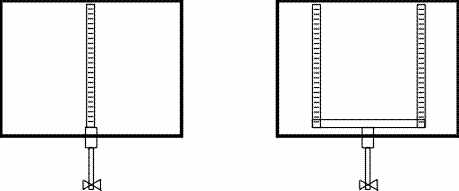
Here is a top view of the manifold layouts:
Initial tests were done by injecting food coloring directly into the mash near the walls and observing the flow paths to the drain. The tests showed a parabolic path to the drain, with faster flow of dye in regions directly above and immediately adjacent to the drain versus dye placed out near the walls several inches away. The results disagreed with our initial drainage model and it was difficult to glean much information from this method. It caused a re-examination of the test procedure.
The next set of experiments involved dying the whole water layer above the grainbed, opening the drain, and watching how the dye flowed into the grainbed. These results were much more telling of the way that sparging actually worked. After all, during the sparge, we are attempting to move fluid through all regions of grainbed to the drain and thereby achieve the best extraction. These experiments showed that there was a big difference in the flow rate, and thus the volume of water, that moved through the bed to the drain from areas above and adjacent to the drain compared to regions far away at the corners.
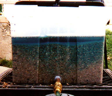
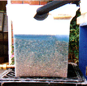
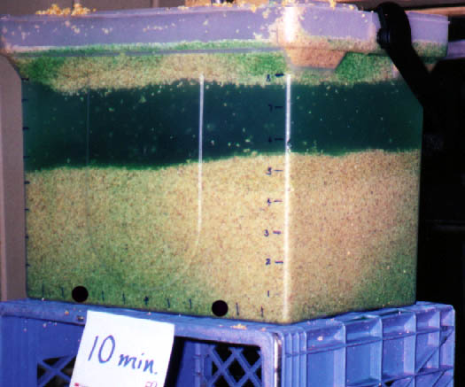
Here are a series of pictures showing how the dye moves through the grainbed toward a single drain:
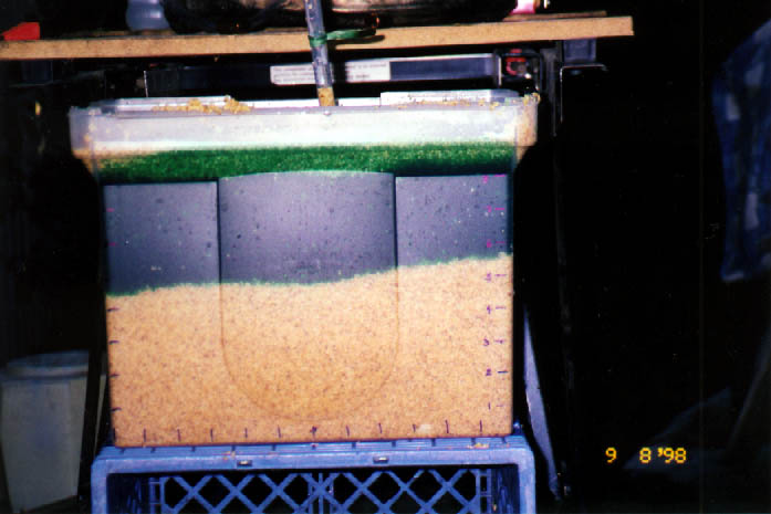
1. This shows the dye above the grainbed prior to opening the drain (in back).
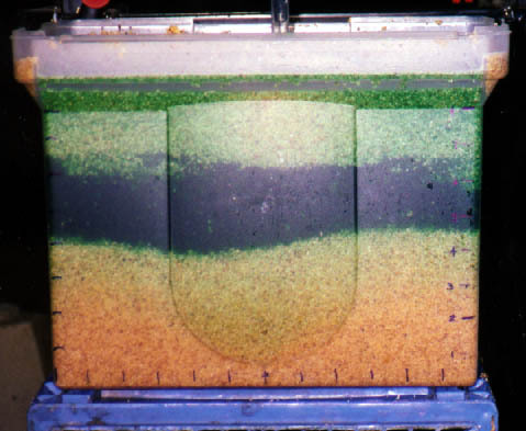
2. This shows flow toward a single drain after about 2 minutes of flow. Note the coning of the dye front. A view from the side better shows the lack of dye to the bottom corner.
<

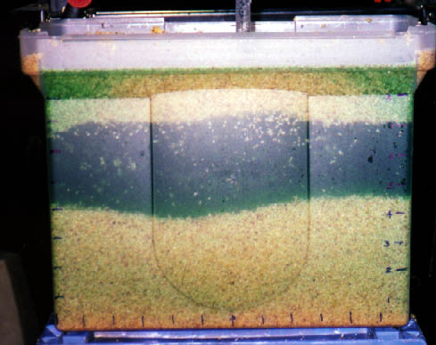
3. After 10 minutes, the dye has reached to within a half inch of the floor, but if you look closely, you can see that the middle area above the drain is starting to rinse clean already. Further observation showed this more clearly, but I ran out of film. As the sparging progressed, the far corners remained green while the center was rinsed clean.
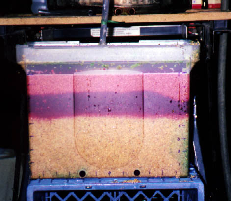
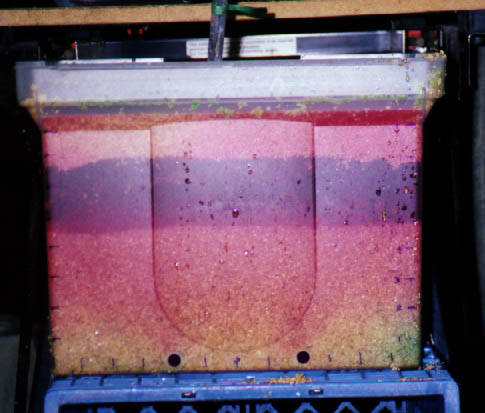
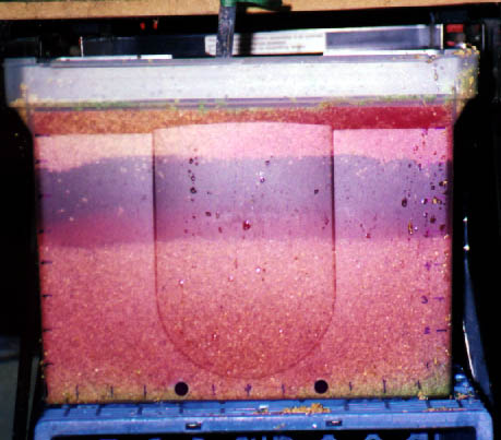
Here are two pictures showing identical behavior in a spent mash with a fair amount of sugar left. (1.015). The temperature of the mash was about 120F during the test, but I was lautering with 90F water, so it was cooling further.
Other trials where flow rate or fluid depth were varied showed no significant difference in behavior of the dye front. Flow rate was tested at 2.2 quarts per minute and 0.5 quart/minute. The dye front moved faster or slower, but was the same shape. Varying the depth of the water, ie. the head height, seemed to change the angle of the cone a bit, but it was hard to tell.
Dual Drains and Spacing
The next round of experiments used two pipes connected to the bulkhead fitting with a Tee. The spacing between the two pipes could be varied. Trials were conducted with spacings of L = 4 and L = 6 inches. These spacings were chosen because the spacing of 6 inches in the 12 inch wide box results in a distance of L/2 between the pipe and the wall, while L = 4 equates to a distance L to the wall. We have suggested L/2 spacing in the past to minimize the affect of preferential flow down the walls of the tun, bypassing the grainbed. (However, due to the actual width of the tubes in this set-up, the distance to the wall was actually 2.5 inch instead of 3 inches.) The two spacings provided a good difference in predicted behavior.
These trials had the following results (black circles are used to indicate drain positions):
1. With the pipe spacing at L=6, the dye front after 2 minutes of flow looked like this:

2. After ten minutes of flow, the dye front had reached the bottom, and the corners were already being rinsed. As mentioned, the spacing of the pipes to the walls is actually less than L/2. The residual color in the back corner of the tun is due to the position of the drain pipe there. Due to the length of the Tee fitting and the elbow fitting, the slotted pipe sits about 2 inches off from the back wall, whereas in front, it comes to within a half inch of the wall.
The next trial was with L = 4, and it looked like this:
1. Before Flow. (some green is left over from the previous trial)
2. After 2 minutes.
3. After 10 minutes. Note some lack of flow at the corners.
Time For A New Model
Obviously, this data did not support the R^2 = 2H^2 model, or vice versa. I started thinking about what this data meant; specifically how to account for the differences in flow rate between different regions.
I realized that the difference in flow velocity for two distances from the drain pipe, r1 and r2, must differ as a function of r^2, rather than just r (linearly). I bounced this hypothesis off Guy, and he agreed that, at the same depth or Head, that v1/v2 = r1^2/r2^2.
Eureka! So, the flow velocity potential at any point in the grainbed is a function of the Head, divided by the distance from the drain (squared). V~ H/r^2 This brought to mind Ohm's Law, which states that the Potential (V) divided by the Resistance (R ) in this case the grainbed and all subsequent plumbing, equals the Current (I) which in this case can be considered as the final flow velocity. It became apparent to me that by plotting the potential for flow across the dimensions of the lauter tun, I could model how the flow reacted to the position of the drain.
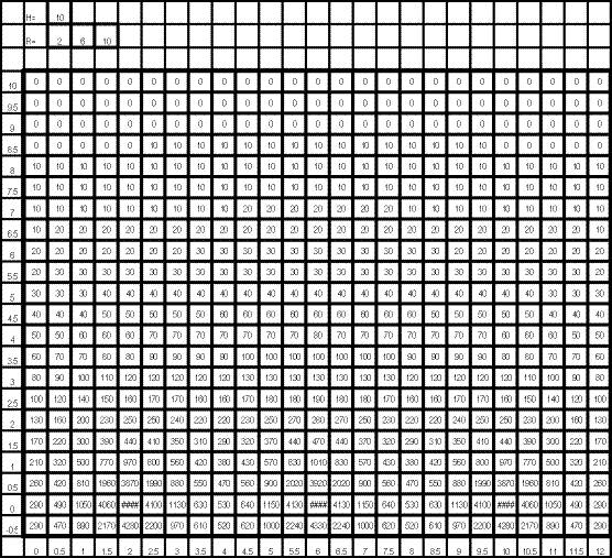
The equation looks like this V = 100H/(x^2+y^2)
The scaler of 100 was used to make V greater than 1 in all cases.
With this idea in hand, I generated an Excel spreadsheet such that the cells each represented a actual square inch and calculated V for that cell's position relative to the drain. The drain was located at the bottom of this "tun", in the middle. The numbers immediately gave an indication of the convergence of the flow I had observed in the trials. I shaded similar values to help indicate this, and the result is below.
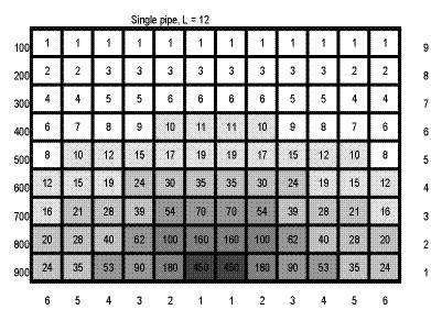
Two drains at L=6 looked like this:

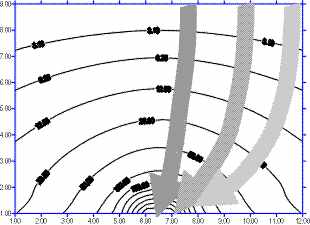
I made up several spreadsheets for single and double drains and sent them to Guy. He agreed with the model, saying it looked like I had succeeded in solving 2D Steady State Flow without resorting to Finite Difference Analysis techniques. He was able to verify it using 3D Flow Modeling software that they have for modeling watersheds. In addition, he was able to take the spreadsheet values and generate equipotential flow gradient lines. These equipotential graphs match the observed flow patterns almost exactly. The graphs are shown below with gray arrows to show how the flow is vectored perpendicular to the gradient lines to approach the drains.
Single drain:
Dual drain:
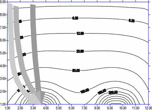
Three drains:
Three drains spaced at 2, 6 and 10 in a 12 inch wide tun work even better than two drains. This spreadsheet is not to scale, nor is it shaded but you can look at the numbers and get the idea.
The spreadsheets show that with the increase in drains, you flatten the equipotential lines across the tun. Increased grainbed depth also helps because it means that a greater percentage of the grain is up in the lesser gradient levels where the equipotential lines are flatter. This model is most applicable to rectangular picnic coolers since they allow a uniform 2D slice.
Custom Designing Your Manifolds
What I hope to do soon is to be able to have a Java applet on my web page which will take the tun dimensions, depth and the drain locations and generate a graph of the equipotential curves. One of the programmers here at work is looking into it.
Further Experimentation Needed
As with any theory and model, there is always more work to be done. As noted above - this model only looks at flow from a Potential aspect. It assumes that the media (grainbed) is homogenous i.e., that the resistance to flow in all cases is the same. In a real mash, this is obviously not the case. Noonan shows in Brewing Lager Beers that a cross-section of the mash has different particle sizes from top to bottom. In fact, during the trial using a spent mash, I had almost a half inch of that annoying topdough on top of the grainbed. It really slowed down the initial flow, even though the shape of the dye front matched what was observed using corncobs.
Wort, by virtue of being more dense than water, and more viscous, will tend to underperform predictions based on water (see the Bernoulli equation) but basically all things being equal (head, temperature, etc.), a thicker denser fluid (syrup) flows through a small pore more slowly than a thinner, lighter one (water). With this in mind, you can hypothesize that as the sparge progresses, the difference in flow rate between the area over the drain versus the areas away from the drain will actually increase due to the increasing difference in wort viscosity and density between the two regions, which should affect extraction. More data is needed in this area.
I think that one aspect of lauter tuns that allows this model to work is that the greatest constraint to flow is at the valve where we meter the flow rate, not within the grainbed. This difference provides for any inhomogeneities in the grainbed to be insignificant compared to resistance downstream. It also allows for all segments of the manifold to draw equally from the bed.
It seems we can’t find what you’re looking for. Perhaps searching can help.